Published 16 November 2016

The field of journey planners has sprung to life over the few last years. Papers from universities released in cooperation with Microsoft and Google have breathed life into a field that was relying on Dijkstra and A* for nearly 40 years. I’ve previously written about the Connection Scan Algorithm and Transfer Patterns, in this post I’m going to take a look at a new journey planning algorithm called Trip Based Public Transit Routing.

The basis of the algorithm is to precalculate useful transfers between trips in order to speed up real time queries. While it’s not strictly a graph based algorithm it’s essentially a breadth first search across a graph using trips as nodes and transfers between them as edges. The algorithm is bicriteria by nature and evaluates both arrival time and number transfers.

Unlike the Transfer Pattern pre-calculation the transfers are not specific to any origin and destination making them a lot faster to compute, not to mention use less space.

The paper itself is well written and this post supplements it with my observations rather than replaces it, if you are looking at implementing the algorithm I recommend you read both. For a TL;DR summary of the algorithm skip to the end.

Before we are able to perform a query the paper describes three preprocessing steps required to generate the transfers used in the main algorithm, but before tackling that we need to group trips into Lines to enable the generation of transfers.

Line Generation

A Line is a set of trips that follow the exact same stopping pattern but do not overtake each other. An example of a Line would be a service that runs many times a day along the same set of stops.

It’s also worth noting that throughout this algorithm interchange is calculated as a footpath from the station to itself, depending on your data source you may need to do some conversion.

To store the lines I set up a map with the signature Map<StoppingPattern, Line[]>. The StoppingPattern is just a string concatenation of the stop stations, for example a Trip(A:1000, B:1015, C:1020) has a stopping pattern of “ABC” with times 1000, 1015, 1020. As stated above overtaken trains are split into new lines so one pattern has a list of Lines.

After setting up the map, group the trips by stopping pattern into another, temporary map of Map<StoppingPattern, Trip[]>. We can then iterate this map and create a Line for each stopping pattern. When adding a trip to a line we must check whether it overtakes any of the services in the line. If it does we split it out into it’s own line.

Generating Transfers

Once we have generated our Lines we iterate over each trip and trips stops to find possible transfers. We exclude the first stop of each trip as you wouldn’t transfer from your origin to another trip - you would board that trip directly at the origin station.

As we iterate the stops we create a set of tuples (arrival time, station) by returning all stations connected via footpath. The arrival time is the arrival time at the original stop + the footpath duration. As interchange time is treated as a footpath from A->A the original stop is included with interchange time applied.

For each of our tuples we check which lines pass through the station and which, if any, trips are reachable at that time. We exclude any transfers that would put us at the destination of the trip we transfer to as you only want to make a transfer if it takes you somewhere new. We only need to transfer to the first reachable trip of the line - as there are no overtaken trains on the same line the first reachable will also be the one that arrivals first at all subsequent stops along the line.

There are a couple of finer points of the algorithm in the paper that took me a while to understand. If the trip you are transferring to belongs to the same line the transfer is only useful in two situations; if the trip you are transferring to arrives before your current trip or the stop you are transferring to is further along the line. It is difficult to imagine situations where this might be the case but sometimes theoretically a footpath may connect you with a stop further along the line in time to reach an earlier service. The other scenario is if the stop you are transferring to is an earlier stop on the line. Though I don’t know why you would want to go back to an earlier station only to board a later service on the same line.

The basic structure I used for a transfer was: Transfer(TripT, StopI, TripU, StopJ).

Removing U-Turn Transfers

The set of transfers generated is quite large. Before doing a journey plan we need to remove any transfers that won’t ever be useful. U-turn transfers, where the transfer takes you back to the proceeding stop of your current trip are not usually helpful. However they may be helpful if you can’t perform your transfer at that preceding stop. This is another area I struggled with for a use case but with some help I managed to find one.

Given two trips in opposite directions it can be beneficial to keep the transfer if they branch later on but transfer is not possible at later stops due to interchange time.

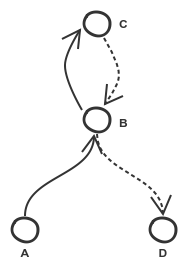
In this example there is a TripT(A,B,C) and a TripU(C,B,D) and a Transfer(TripT, C, TripU, C) the transfer is kept if and only if interchange is not possible at B because of a large interchange time. I think it’s probably quite a rare occurrence but definitely possible.

It’s not necessary to check that the lines branch but that is the only logical scenario I could think of.

The code for step one and step two can be combined into a single process. The number of nested for loops is quite hideous bit the context is required all the way down. Without for-comprehensions there’s no pretty way of doing it.

Removing Transfers That Don’t Improve Arrival Time

The final step of pre-calculation is to iterate through each trip and work out which of its transfers lead to a better arrival time at any particular station.

For each trip we set up two indexes; the best arrival time for each station and the best departure time from each station.

Working backwards through the trip’s stops (again excluding the first stop on the trip as it won’t transfer anywhere) we check any possible transfers. For each stop along trip after the transfer we check to see if it improves the arrival/departure time at any station, if so we keep it. It may seem obvious but it’s worth noting that we only check stops on TripU of the transfer after StopJ otherwise we’d be going backwards along the line, and possibly into the past.

Earliest Arrival Queries

As stated earlier the actual query itself is a breadth first search using trips as nodes and transfers as edges. Before beginning the search we set up two data structures:

The first is a map of trips that arrive at the destination or a station connected to the destination by footpath. The trip is the key of the map and the value is a tuple of (Line, stopIndex, footpathTime).

The second is a nested queue of trip segments to scan. A trip segment is a subsection of a trip denoted by TripSegment(Trip, stopI, stopJ). The different levels of the queue correspond to the number of transfers required to get to that trip segment so we initially seed it with all trips possible from the origin station, or a station connected to the origin station by footpath at level 0 (no transfers).

As we scan each trip segment we check if the trip is one of those in our first data structure (and therefore connected to the destination). If it is, check if the first stop of the trip segment occurs before the destination stop. As the destination station is on the trip it will definitely be reachable but we only want to add the journey if it improves the arrival time. Assuming it does improve the arrival time we add it to our list of results and remove any other results we stored that are no longer relevant (the paper describes these as dominated).

Regardless of whether we found a result when checking the trip segment we want to add any transfers possible on the current trip segment to the queue. Given that we are making a transfer we actually add any trip segments we are going to scan to the next level of the queue. As we add items to the queue we maintain an index of trips and the earliest stop on the trip we’ve examined. We can ignore any trip segments added to the queue that don’t add any earlier stops as they will already have been scanned or already be in the queue.

After we’ve scanned all of the trip segments on the current level of the queue we jump to the next one and repeat the process until there are no more levels to jump to. The paper actually states they cap the maximum number of transfers at 15 as there were no useful journeys in their data set after 15 transfers, your milage may vary.

You’ll also note that the default implementation just returns the arrival time, which by itself is not much use. In order to turn the arrival time into a journey we need to store the preceding trip every time we add a journey segment to the queue. This way we can iterate backwards through the journeys legs and build up a full itinerary.

I split out the implementation of the queue but the breadth first search looks like this:

Observations

I would say that this is a very robust algorithm, the way it deals with interchange time and footpaths is quite elegant. Overtaken trains have also been accounted for which tells me that the algorithm has actually been given a good run though with real world data. The fact that it is bicriteria by nature is also a bonus.

The biggest issue I struggled with was what to do with trips that only run between certain dates. In general GTFS timetables deal with dates and times separately in order to reduce the number of services. I contacted Dr Sascha and his suggestion was to calculate the transfers for each day separately. This is a reasonable compromise as the calculation time is quite quick, the paper states a 8-core processor takes about 2 minutes for the German national data. My single-core implementation of the UK GTFS feed takes about 40 minutes (it is written in node). The only issue that this then raised was that performing a query must be done with only the lines and transfers for that specific day. Unless you have more memory than you know what to do with this becomes inefficient. As a work around I loaded the trips and transfers for a specific day and only passed those to the breadth first search. This increased the query time significantly.

Doing a query takes roughly 20 seconds but almost all of this time is spent loading the data. If I was able to store each day’s trips and transfers in memory I could get the results in well under a second in most cases.

The paper’s implementation of the algorithm does make use of some heavily optimized C++ to get some good query times. My implementation in TypeScript performed poorly in both memory consumption and time taken. TypeScript (node.js) is not a good language for this type of work but it is quite nice to flesh out ideas and get in idea of how the algorithm works. I would be interested in implementing it in a more appropriate language to see if I can cut down the loading time.

In terms of complexity I would say this algorithm is much harder to implement that the Connection Scan Algorithm or Transfer Patterns but it’s worth bearing in mind that Transfer Patterns require another journey planning algorithm for processing and the Connection Scan Algorithm only evaluates earliest arrival time and not number of transfers.

There is a follow up paper that incorporates a transfer pattern style preprocessing step and it’s possible this would solve the issues I was seeing with loading time as I could loada much smaller set of data when performing the query.

My rough and ready TypeScript implementation is available on github.

Acknowledgements

It’s fair to say I had a lot of help implementing this algorithm so I’d like to thank Mike Kazantsev for guiding me through a lot of it.